TL;DR

Transformer模型为了处理序列的位置信息，引入了位置编码(Position Embedding, PE)。常见的位置编码方案有绝对位置编码(Absolute Position Embedding)、相对位置编码(Relative Position Embedding)和旋转位置编码(Rotary Position Embedding, RoPE)。

绝对位置编码：使用三角函数式位置编码，如Sinusoidal APE，将位置信息累加到输入序列的元素向量中，有助于模型感知输入的顺序。
相对位置编码：不为每个元素引入特定的位置表征，而是关注元素之间的相对位置关系。在NeZha、DeBERTa等模型中使用，有更强的长距离依赖建模能力。
旋转位置编码：是在绝对位置编码的基础上引入的一种改进，采用了“绝对位置编码方式实现的相对位置编码”，在实验中表现出更好的性能。

针对模型处理长文本的问题，提出了几种长度外推方法：

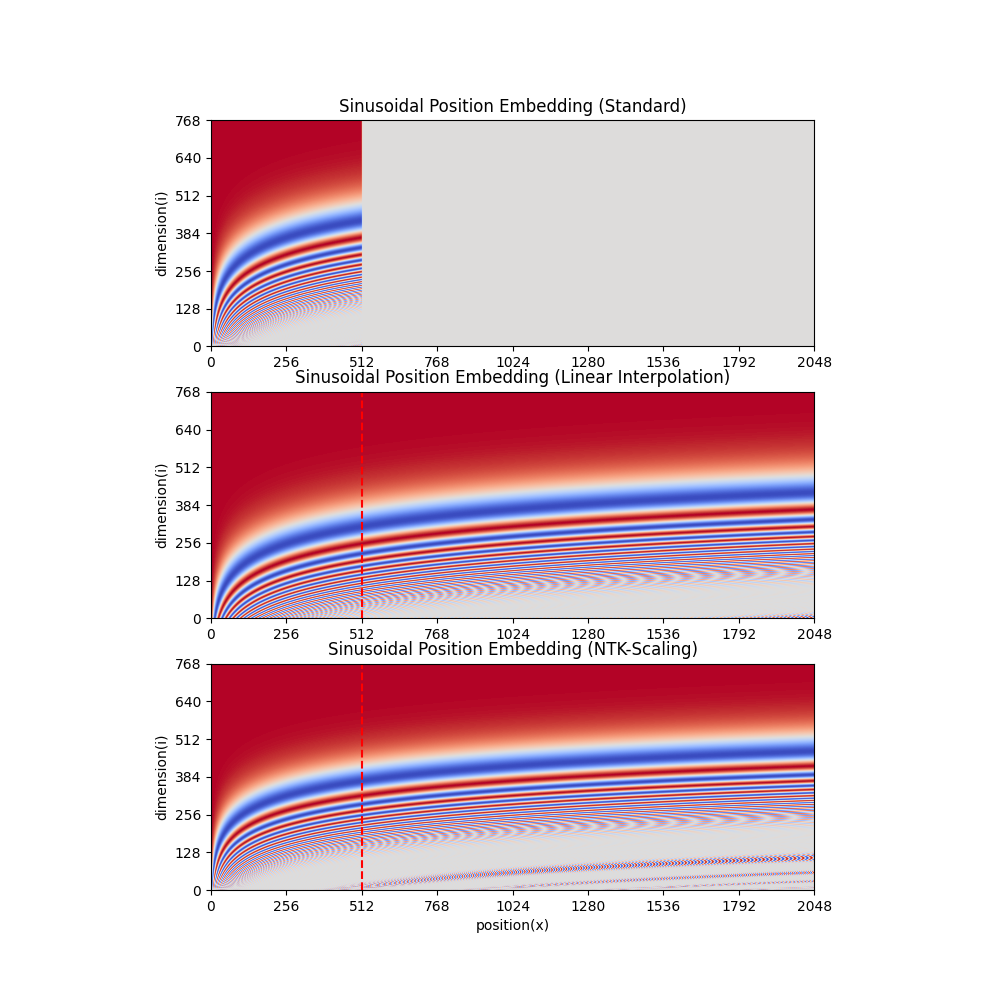
线性内插（Linear Interpolation）：通过减小位置精度，使得可表示范围内容纳更多位置，但可能需要进一步预训练适配。
NTK-Scaling RoPE：通过非线性插值，改变RoPE的基数而不是缩放，以保持位置精度，适用于不经过微调即可具有良好长度外推能力。
Dynamically NTK-Scaling RoPE：在NTK-Scaling RoPE的基础上，根据输入长度按需动态调整缩放系数，从而取得外推长度和位置精度之间的平衡，提高适应性。

这些方法可以帮助模型在处理长文本时更好地维护位置关系，提高性能。几种长度拓展方法的对比图（横轴是序列位置、纵轴是维度）如下：

Transformer中的位置编码

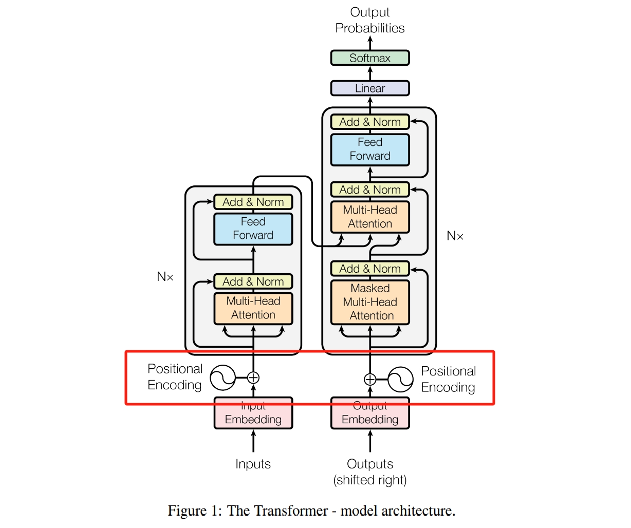
传统的序列建模模型——循环神经网络(Recurrent Neural Network, RNN)迭代式地完成序列建模，也就是说各元素依次输入到模型中计算词向量表征，因而天然地引入了位置信息；而Transformer是将序列一次性输入模型，由注意力机制完成元素间的全局依赖建模。这种方式的优点是可以并行地处理序列，从而提高计算资源利用率、加速模型运算，缺点是元素对之间的计算是独立的，导致了位置关系的丢失，可能产生由语序导致的语义混乱，比如“小明喜欢狗但不喜欢猫”和“小明不喜欢狗但喜欢猫”两句话的词向量表在数值上是完全一致的。

为了解决以上问题，Transformer模型引入了位置编码嵌入。现在常见的位置编码方案有绝对位置编码、相对位置编码、旋转位置编码等。

绝对位置编码 是将位置信息编码为固定长度的向量，累加到输入序列对应位置的元素向量表征上。这样可以在保留元素信息的同时，将位置信息融入到表征中，从而帮助模型感知到输入的顺序。Attention Is All You Need一文提出Transformer结构时，采用了固定的三角函数式位置编码(Sinusoidal APE)，如下：

$\begin{equation} \begin{cases} P(i, 2d) &= \sin (i / 10000^{2d / d_k}) \\ P(i, 2d + 1) &= \cos (i / 10000^{2d / d_k}) \end{cases} \end{equation}$

其中， $i$ 是位置索引、 $d$ 是维度索引、 $d_k$ 是表征向量的维数，因此 $P \in \mathbb{R}^{l \times d_k}$ ， $l$ 是序列长度。BERT模型将三角函数式位置编码调整为了可训练的位置编码，从而使模型根据数据特点自适应地调整位置编码，以帮助模型更好地理解句子中单词的相对位置关系、提高模型在各种自然语言处理任务中的性能。这一改进使得BERT在处理长文本和长距离依赖关系时表现更加出色。

相对位置编码 相对位置编码没有为每个元素引入特定的位置表征，而是更关注元素之间的相对位置关系。在不同长度的输入下，不会产生位置原因导致的参数收敛速度差异，因而具有更好的泛化性^参数收敛速度差异。另外，与绝对位置编码相比，相对位置编码具有更强的长距离依赖建模能力，能更好地处理长序列。使用相对位置编码的典型模型有NeZha、DeBERTa。下面是NeZha采用的相对位置编码计算方式，是在计算Attention Score时引入位置信息：

$\begin{equation} \begin{aligned} a_{ij} &= \text{softmax}(\frac{q_i^\top (k_j + R^{K}_{ij})}{\sqrt{d_k}}) \\ o_i &= \sum_j a_{ij} (v_j + R^{V}_{ij}) \end{aligned} \end{equation}$

其中， $q_i$ 是 $x_i$ 对应的查询向量、 $k_j$ 、 $v_j$ 是 $x_j$ 对应的键值向量， $R^{*}_{ij} \in \mathbb{R}^{d_k}$ 是 $x_i$ 和 $x_j$ 间距离对应的相对位置向量，一般采用固定的三角函数式位置编码。值得注意的是，每一层Attention计算时都会引入相对位置编码，也就是说每一层都会强化位置信息，这能防止深层网络层丢失位置信息，这可能也是比绝对位置编码效果更好的原因之一。

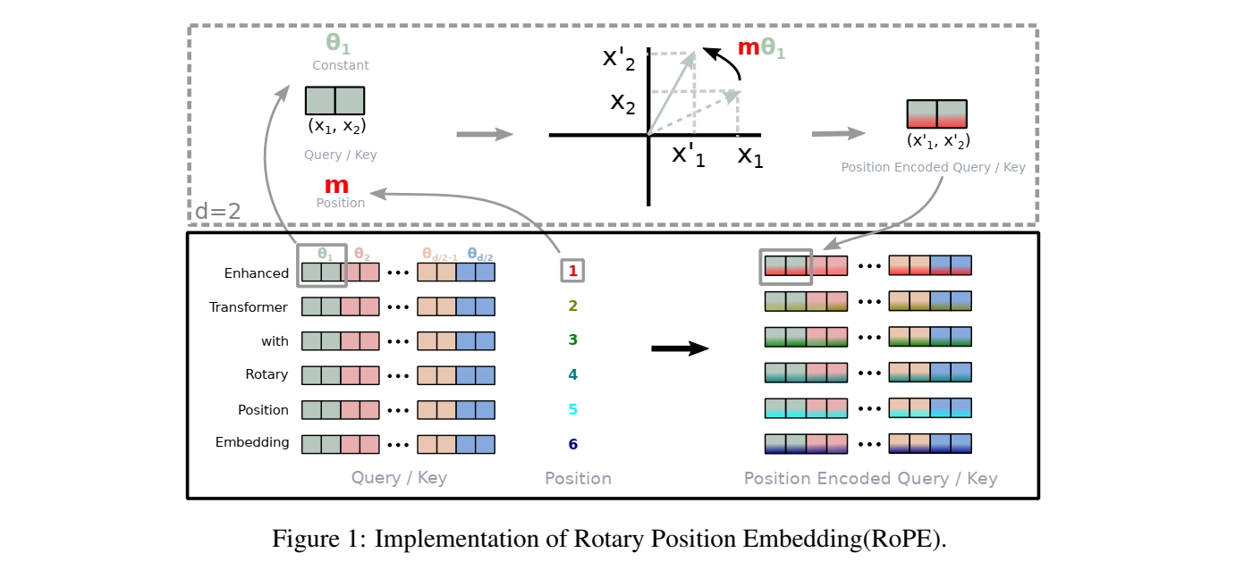
旋转式位置编码 旋转式位置编码由苏剑林在其博客Transformer升级之路：2、博采众长的旋转式位置编码中首次提出，后在Roformer论文中正式定义。旋转式位置编码是一种“绝对位置编码方式实现的相对位置编码”，是指计算方式上与绝对位置相似，但实际效果是考虑的元素间的相对位置信息。实验效果证明该方法能带来更好的模型性能，被目前主流大语言模型所广泛采用。

$\begin{equation} f(x, i) = \begin{bmatrix} x_0 \\ x_1 \\ x_2 \\ x_3 \\ \vdots \\ x_{d_k - 2} \\ x_{d_k - 1} \end{bmatrix} \odot \begin{bmatrix} \cos i\theta_0 \\ \cos i\theta_0 \\ \cos i\theta_1 \\ \cos i\theta_1 \\ \vdots \\ \cos i\theta_{d_k / 2 - 1} \\ \cos i\theta_{d_k / 2 - 1} \\ \end{bmatrix} + \begin{bmatrix} - x_0 \\ x_1 \\ - x_2 \\ x_3 \\ \vdots \\ - x_{d_k - 2} \\ x_{d_k - 1} \end{bmatrix} \odot \begin{bmatrix} \sin i\theta_0 \\ \sin i\theta_0 \\ \sin i\theta_1 \\ \sin i\theta_1 \\ \vdots \\ \sin i\theta_{d_k / 2 - 1} \\ \sin i\theta_{d_k / 2 - 1} \\ \end{bmatrix} \end{equation}$

其中 $x$ 是输入对应的向量表征， $i$ 是指该向量在序列中的位置， $\theta \in \mathbb{R}^{d_k/2}$ 是常数向量， $\theta_d = 10000^{-2d/d_k}$ 。

位置编码存在的问题 但不管是绝对式位置编码还是相对式位置编码，都是基于一组预定义的位置向量编码训练的。因此当文本长度超出了这个编码表所能表示的范围时，位置编码就无法正确地表达文本中各个位置之间的关系，从而影响模型对长文本的处理能力。因此，目前语言模型模型的长度外推是非常值得研究的、具有重大现实意义的问题。

鉴于目前主流大语言模型都采用了RoPE，本文介绍的几种方法都是基于RoPE的。有兴趣的读者也可以查看苏剑林在对绝对位置编码进行长度外推的尝试：层次分解位置编码，让BERT可以处理超长文本。

旋转位置编码的性质

上文介绍到RoPE中 $\theta$ 借鉴了正余弦位置编码：

$\begin{equation} \theta_d = 10000^{-2d/d_k} \end{equation}$

$d \uparrow \Rightarrow \theta_d \downarrow$ ，对于 $d \geq 0$ ， $0 < \theta_d \leq 1$ ，那么 $0 < i \theta_d \leq i$ 。

代入正弦三角函数有

$\begin{equation} \sin i \theta_d = \sin \left( 10000^{-2d/d_k} \cdot i \right) \end{equation}$

与正弦三角函数的一般形式 $y = A \sin (\omega t + \phi) + C$ 比较，我们可以得到：

$\begin{equation} \omega = \theta_d = 10000^{-2d/d_k} \end{equation}$

当 $d \uparrow \Rightarrow \omega \downarrow$ ，即维数越高、频率越低，这就类似数学进制中从个位到十位、百位、…的关系。苏剑林也在 Transformer升级之路：10、RoPE是一种β进制编码 中指出RoPE实际上是一种特定的 $\beta$ 进制编码， $\beta = 10000^{2/d_k} \Rightarrow \theta_d = \beta^{-d}$ ：

$\begin{equation} \begin{aligned} & \begin{bmatrix} \cos i\theta_0 & \sin i\theta_0 & \cos i\theta_1 & \sin i\theta_1 & \cdots & \cos i\theta_{d_k / 2 - 1} & \sin i\theta_{d_k / 2 - 1} \end{bmatrix} \\ = & \begin{bmatrix} \cos \frac{i}{\beta^0} & \sin \frac{i}{\beta^0} & \cos \frac{i}{\beta^1} & \sin \frac{i}{\beta^1} & \cdots & \cos \frac{i}{\beta^{d_k / 2 - 1}} & \sin \frac{i}{\beta^{d_k / 2 - 1}} \end{bmatrix} \end{aligned} \end{equation}$

有意思的解释一下，RoPE 的行为就像一个时钟。12小时时钟基本上是一个维度为 3、底数为 60 的 RoPE。因此，每秒钟，分针转动 1/60 分钟，每分钟，时针转动 1/60。—— 浅谈LLM的长度外推 - 知乎

几种长度外推方法

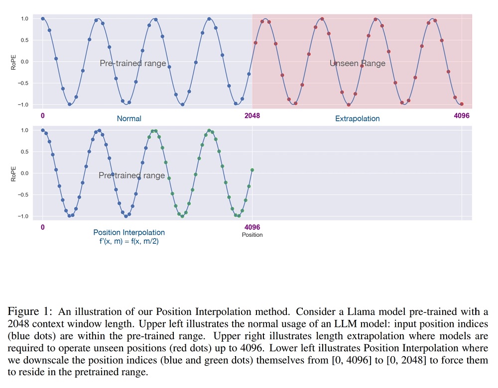
Linear Interpolation 线性内插式，由Meta发表在论文 EXTENDING CONTEXT WINDOW OF LARGE LANGUAGE MODELS VIA POSITION INTERPOLATION 上，另一篇博客 Extending Context is Hard…but not Impossible 也提到了这种方法。是在不改变已有位置编码可表示范围的前提下，压缩位置精度，使可表示范围内可容纳更多的位置。举个例子，一条100米的路隔1米种1棵树能种100棵树，现在要在这100米的路上种下400棵树，那么就每隔0.25米种1棵树。

$\begin{equation} i' = i / scale \end{equation}$

那么最多可表示 $20418$ 序列长度的位置编码范围，就能容纳 $2048 \times scale$ 个序列元素。该方法的优点是实现简单，缺点是需要进一步预训练来使模型适配内插的位置编码。另外，该方法会损失位置的表示精度，过大的缩放尺度可能导致模型效果不佳，Meta也在论文中说明该方法在拓展上下文时存在约600x的上限[^线性内插缩放上限]。使用这种方法的典型模型是LongChat。🤗transformers库中LLaMA模型LlamaLinearScalingRotaryEmbedding的具体实现如下：

    def _set_cos_sin_cache(self, seq_len, device, dtype):
        self.max_seq_len_cached = seq_len
        t = torch.arange(self.max_seq_len_cached, device=device, dtype=self.inv_freq.dtype)
+       t = t / self.scaling_factor

        freqs = torch.outer(t, self.inv_freq)
        # Different from paper, but it uses a different permutation in order to obtain the same calculation
        emb = torch.cat((freqs, freqs), dim=-1)
        self.register_buffer("cos_cached", emb.cos().to(dtype), persistent=False)
        self.register_buffer("sin_cached", emb.sin().to(dtype), persistent=False)

[^线性内插缩放上限]: Our theoretical study shows that the upper bound of interpolation is at least ∼ 600× smaller than that of extrapolation, further demonstrating its stability.

NTK-Scaling RoPE 在reddit论坛的文章 NTK-Aware Scaled RoPE allows LLaMA models to have extended (8k+) context size without any fine-tuning and minimal perplexity degradation. 上首次提出，目的是希望在进行长度外推的同时，保持位置编码的精度。

Instead of the simple linear interpolation scheme, I’ve tried to design a nonlinear interpolation scheme using tools from NTK literature. Basically this interpolation scheme changes the base of the RoPE instead of the scale, which intuitively changes the “spinning” speed which each of the RoPE’s dimension vectors compared to the next. Because it does not scale the fourier features directly, all the positions are perfectly distinguishable from eachother, even when taken to the extreme (eg. streched 1million times, which is effectively a context size of 2 Billion).

前面说到，RoPE可以视作 $\beta$ 进制，如下

$\begin{equation} \begin{aligned} & \theta_d = 10000^{-2d/d_k} \\ \Rightarrow & \theta_d = \beta^{-d}, \beta = 10000^{2/d_k} \end{aligned} \end{equation}$

为了保证位置精度不变，NTK-Scaling 没有改变低维的高频编码，而随着维数升高逐步地增大线性内插的比例，即 $i \uparrow \Rightarrow scale \uparrow$ ，从而增大整体可表示位置范围。为了实现该目标，引入参数 $\alpha > 1$ 指数增加插值比例，即越低频的维度插值比例越高：

$\begin{equation} \theta_d' = (\alpha \beta)^{-d} \end{equation}$

可表示范围受最低频维度限制，因此在最高维（最低频）实现 $scale$ 倍的线性内插，即

$\begin{equation} \begin{aligned} & \theta_{d_k/2-1}' = \theta_{d_k/2-1} / scale \\ \Rightarrow & \frac{1}{(\alpha \bcancel{\beta})^{\frac{d_k}{2} - 1}} = \frac{1}{scale} \frac{1}{\bcancel{\beta^{\frac{d_k}{2} - 1}}} \\ \Rightarrow & \alpha = scale^{\frac{2}{d_k - 2}} \end{aligned} \end{equation}$

因此

$\begin{equation} \begin{aligned} \theta_d' &= (\alpha \beta)^{-d} \\ &= (\beta \cdot scale^{\frac{2}{d_k - 2}})^{-d} \\ &= (10000^{\frac{2}{d_k}} \cdot scale^{\frac{2}{d_k - 2}})^{-d} \\ &= \underline{(10000 \cdot scale^{\frac{d_k}{d_k - 2}})}^{-2d / d_k} \end{aligned} \end{equation}$

实际中，通过scale参数计算得 $\alpha$ ，然后修改底数base实现。

    def _set_cos_sin_cache(self, seq_len, device, dtype):
        self.max_seq_len_cached = seq_len

+       if seq_len > self.max_position_embeddings:
+           base = self.base * self.scaling_factor ** (self.dim / (self.dim - 2))
+           inv_freq = 1.0 / (base ** (torch.arange(0, self.dim, 2).float().to(device) / self.dim))
+           self.register_buffer("inv_freq", inv_freq, persistent=False)

        t = torch.arange(self.max_seq_len_cached, device=device, dtype=self.inv_freq.dtype)

        freqs = torch.outer(t, self.inv_freq)
        # Different from paper, but it uses a different permutation in order to obtain the same calculation
        emb = torch.cat((freqs, freqs), dim=-1)
        self.register_buffer("cos_cached", emb.cos().to(dtype), persistent=False)
        self.register_buffer("sin_cached", emb.sin().to(dtype), persistent=False)

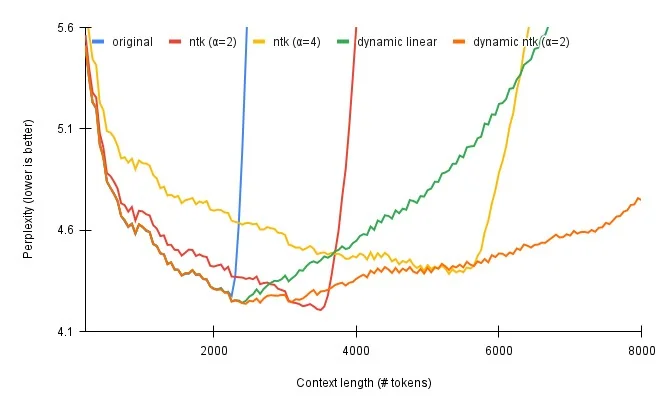
实验效果如下（未经过微调），可以看到随着 $\alpha$ 增大( $2 \rightarrow 4 \rightarrow 8 \rightarrow 16$ )，虽然短文本混淆度(Perplexity, PPL)上升，但长文本的PPL获得的PPL收益更为显著，而且不经过训练也能具有良好的长度外推能力，相信通过进一步训练能取得比线性内插更好的效果。

注意，由于位置编码是随着序列长度变化的，文本生成过程中需要保证已缓存的Q、K、V张量与新生成token的保持一致，具体做法是每新生成一个token时都需要根据新的文本长度更新位置编码。

Dynamically NTK-Scaling RoPE Dynamically Scaled RoPE further increases performance of long context LLaMA with zero fine-tuning 一文中提出的对NTK-Scaling RoPE的改进，与NTK-Scaling RoPE使用固定 $\alpha$ 参数不同，Dynamically NTK-Scaling RoPE能根据输入长度动态地调整 $\alpha$ ，从而实现按需调整缩放系数。

$\begin{equation} \begin{aligned} \theta_d' &= \left( 10000 \cdot \underline{(\frac{l}{l_{max}} \cdot scale - (scale - 1))}^{\frac{d_k}{d_k - 2}} \right)^{-2d / d_k} \end{aligned} \end{equation}$

Qwen-14B-Chat 就采用了这种方式将8k的上下文长度拓展到了32k。

🤗transformers库中LLaMA模型LlamaDynamicNTKScalingRotaryEmbedding的具体实现如下：

    def _set_cos_sin_cache(self, seq_len, device, dtype):
        self.max_seq_len_cached = seq_len

+       if seq_len > self.max_position_embeddings:
+           base = self.base * (
+               (self.scaling_factor * seq_len / self.max_position_embeddings) - (self.scaling_factor - 1)
+           ) ** (self.dim / (self.dim - 2))
+           inv_freq = 1.0 / (base ** (torch.arange(0, self.dim, 2).float().to(device) / self.dim))
+           self.register_buffer("inv_freq", inv_freq, persistent=False)

        t = torch.arange(self.max_seq_len_cached, device=device, dtype=self.inv_freq.dtype)

        freqs = torch.outer(t, self.inv_freq)
        # Different from paper, but it uses a different permutation in order to obtain the same calculation
        emb = torch.cat((freqs, freqs), dim=-1)
        self.register_buffer("cos_cached", emb.cos().to(dtype), persistent=False)
        self.register_buffer("sin_cached", emb.sin().to(dtype), persistent=False)

有意思的解释一下，RoPE 的行为就像一个时钟。12小时时钟基本上是一个维度为 3、底数为 60 的 RoPE。因此，每秒钟，分针转动 1/60 分钟，每分钟，时针转动 1/60。现在，如果将时间减慢 4 倍，那就是二使用的线性RoPE 缩放。不幸的是，现在区分每一秒，因为现在秒针几乎每秒都不会移动。因此，如果有人给你两个不同的时间，仅相差一秒，你将无法从远处区分它们。NTK-Aware RoPE 扩展不会减慢时间。一秒仍然是一秒，但它会使分钟减慢 1.5 倍，将小时减慢 2 倍。这样，您可以将 90 分钟容纳在一个小时中，将 24 小时容纳在半天中。所以现在你基本上有了一个可以测量 129.6k 秒而不是 43.2k 秒的时钟。由于在查看时间时不需要精确测量时针，因此与秒相比，更大程度地缩放小时至关重要。不想失去秒针的精度，但可以承受分针甚至时针的精度损失。—— 浅谈LLM的长度外推 - 知乎

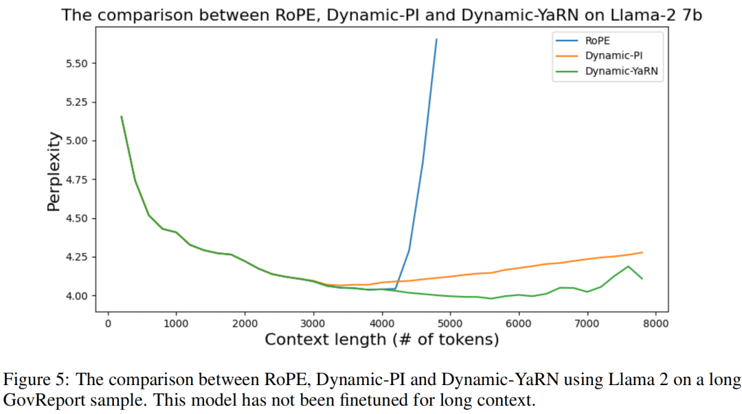
YaRN 无论是线性内插还是NTK类方法，都是通过降低旋转速度来实现长度外推，那么会导致词向量之间的距离变得比原来更近，导致点乘结果变大，从而破坏模型原始的注意力分布注意力。YaRN: Efficient Context Window Extension of Large Language Models 解决方案是在注意力计算时，添加温度系数 $t$ 来修正分布，也就是

$\begin{equation} a_{ij} = \text{softmax}(\frac{(\mathcal{R}_i q_i)^\top (\mathcal{R}_j k_j)}{t \sqrt{d_k}}) \end{equation}$

文中推荐 LLaMA 和 LLaMA 2 的温度系数通过下式求解：

$\begin{equation} \sqrt{\frac{1}{t}} = 0.1 \ln scale + 1 \end{equation}$

The equation above is found by fitting 1/t at the lowest perplexity against the scale extension by various factors s using the “NTK-by-parts” method (Section 3.2) on LLaMA 7b, 13b, 33b and 65b models without fine-tuning.

实验效果如下

参考资料

附：旋转式位置编码推导及具体实现

目标是找到一个函数 $f(x, i)$ （具有初始条件 $f(x, 0) = x$ ），对向量 $q$ 、 $k$ 执行运算后得到带有位置信息的 $\tilde{q}$ 、 $\tilde{k}$ ，希望执行内积运算得到的Attention Score带有相对位置编码，即

$\begin{equation} f(q_i, i)^\top f(k_j, j) = g(q_i, k_j, i - j) \end{equation}$

借助复数求解，那么 $f(x, i)$ 可以表示成

$\begin{equation} f(q_i, i)^\top f(k_j, j) = g(q_i, k_j, i - j) \end{equation}$

复数中满足 $q_i^\top k_j = \text{Re}[q_i^\top k_j^*]$ ， $\text{Re}[\cdot]$ 表示取实部，因此

$\begin{equation} \text{Re}[f(q_i, i)^\top f^*(k_j, j)] = g(q_i, k_j, i - j) \end{equation}$

简单起见，假设存在复数满足

$\begin{equation} f(x, i) = | f(x, i) | e^{\text{i} \phi(i)} \end{equation}$

注意区分上式中 $\text{i}$ 表示虚数单位， $i$ 是位置。根据复数运算，模长和幅角分别有

$\begin{equation} \begin{cases} \begin{vmatrix} f(q_i, i) \end{vmatrix} \begin{vmatrix} f(k_j, j) \end{vmatrix} &= \begin{vmatrix} g(q_i, k_j, i - j) \end{vmatrix} \\ \arg f(q_i, i) - \arg f(k_j, j) &= \arg g(q_i, k_j, i - j) \end{cases} \end{equation}$

令 $i = j$ ，有

$\begin{equation} \begin{cases} \begin{vmatrix} f(q_i, i) \end{vmatrix} \begin{vmatrix} f(k_j, i) \end{vmatrix} &= \begin{vmatrix} g(q_i, k_j, 0) \end{vmatrix} \\ &= \begin{vmatrix} f(q_i, 0) \end{vmatrix} \begin{vmatrix} f(k_j, 0) \end{vmatrix} \\ &= \begin{vmatrix} q_i \end{vmatrix} \begin{vmatrix} k_j \end{vmatrix} \\ \arg f(q_i, i) - \arg f(k_j, i) &= \arg g(q_i, k_j, 0) \\ &= \arg f(q_i, 0) - \arg f(k_j, 0) \\ &= \arg q_i - \arg k_j \\ \end{cases} \end{equation}$

$\begin{equation} \begin{aligned} \Rightarrow \arg f(q_i, i) - \arg q_i = \arg f(k_j, i) - \arg k_j \end{aligned} \end{equation}$

观察等号左右，设

$\begin{equation} \begin{cases} | f(x, i) | &= | x | \\ \phi(x, i) &= \arg f(x, i) - \arg x \end{cases} \end{equation}$

现在 $| f(x, i) |$ 已经有了，接下来求解 $\phi(x, i)$ 。

对于

$\begin{equation} \begin{aligned} \phi(q_i, i) - \phi(k_j, j) &= (\arg f(q_i, i) - \arg q_i) - (\arg f(k_j, j) - \arg k_j) \\ &= \arg f(q_i, i) - \arg f(k_j, j) + \arg q_i - \arg k_j \\ &= \arg g(q_i, k_j, i - j) + \arg q_i - \arg k_j \end{aligned} \end{equation}$

当 $j = i - 1$ 时，有

$\begin{equation} \begin{aligned} \phi(q_i, i) - \phi(k_j, i - 1) &= \arg g(q_i, k_j, 1) + \arg q_i - \arg k_j \\ &= \theta (常数) \end{aligned} \end{equation}$

因此 $\{\phi(i)\}$ 是等差数列，即

$\begin{equation} \phi(i) = i \theta \end{equation}$

所以最终

$\begin{equation} \begin{cases} | f(x, i) | &= | x | \\ \phi(i) &= i \theta \end{cases} \end{equation}$

那么

$\begin{equation} \begin{aligned} f(x, i) &= | f(x, i) | e^{\text{i} \phi(i)} \\ &= | x | e^{\text{i} \cdot i \theta} \end{aligned} \end{equation}$

对于二维向量 $x \in \mathbb{R}^2$ 来说，有

$\begin{equation} \begin{aligned} f(x, i) &= \begin{bmatrix} \cos i \theta & - \sin i \theta \\ \sin i \theta & \cos i \theta \end{bmatrix} \begin{bmatrix} x_0 \\ x_1 \end{bmatrix} \end{aligned} \end{equation}$

该式的物理意义非常明确，是在复平面上将向量 $x$ 逆时针旋转 $i \theta$ 的角度，因此被称作“旋转位置编码”。利用内积的线性叠加性推广到多维（偶数维），有

$\begin{equation} f(x, i) = \mathcal{R}_i x = \begin{bmatrix} \cos i\theta_0 & - \sin i\theta_0 & 0 & 0 & \cdots 0 & 0 \\ \sin i\theta_0 & \cos i\theta_0 & 0 & 0 & \cdots 0 & 0 \\ 0 & 0 & \cos i\theta_1 & - \sin i\theta_1 & \cdots 0 & 0 \\ 0 & 0 & \sin i\theta_1 & \cos i\theta_1 & \cdots 0 & 0 \\ \vdots & \vdots & \vdots & \vdots & \ddots & \vdots & \vdots \\ 0 & 0 & 0 & 0 & \cdots & \cos i\theta_{d_k / 2 - 1} & - \sin i\theta_{d_k / 2 - 1} \\ 0 & 0 & 0 & 0 & \cdots & \sin i\theta_{d_k / 2 - 1} & \cos i\theta_{d_k / 2 - 1} \\ \end{bmatrix} \begin{bmatrix} x_0 \\ x_1 \\ x_2 \\ x_3 \\ \vdots \\ x_{d_k - 2} \\ x_{d_k - 1} \end{bmatrix} \end{equation}$

那么自注意力计算时，位置 $i$ 处的向量 $q_i$ 和 $j$ 处的向量 $k_j$ 计算点积，实现了相对位置编码的引入：

$\begin{equation} \begin{aligned} (\mathcal{R}_i q_i)^\top (\mathcal{R}_j k_j) &= q_i^\top \mathcal{R}_i^\top \mathcal{R}_j k_j = q_i^\top \mathcal{R}_{j - i} k_j \\ &= q_i^\top \begin{bmatrix} \ddots & & & \\ & \cos i \theta_d & - \sin i \theta_d & \\ & - \sin i \theta_d & \cos i \theta_d & \\ & & & \ddots \\ \end{bmatrix}^\top \begin{bmatrix} \ddots & & & \\ & \cos j \theta_d & - \sin j \theta_d & \\ & - \sin j \theta_d & \cos j \theta_d & \\ & & & \ddots \\ \end{bmatrix} k_j \\ &= q_i^\top \begin{bmatrix} \ddots & & & \\ & \cos i \theta_d \cos j \theta_d + \sin i \theta_d \sin j \theta_d & - \cos i \theta_d \sin j \theta_d - \sin i \theta_d \cos j \theta_d & \\ & - \sin i \theta_d \cos j \theta_d - \cos i \theta_d \sin j \theta_d & \sin i \theta_d \sin j \theta_d + \cos i \theta_d \cos j \theta_d & \\ & & & \ddots \\ \end{bmatrix} k_j \\ &= q_i^\top \begin{bmatrix} \ddots & & & \\ & \cos [(i - j) \theta_d] & - \sin [(i + j) \theta_d] & \\ & - \sin [(i + j) \theta_d] & \cos [(i - j) \theta_d] & \\ & & & \ddots \\ \end{bmatrix} k_j \\ \end{aligned} \\ \end{equation}$

为了减少 $\mathcal{R}_i$ 稀疏性带来的冗余计算，写作

考虑远程衰减，采用Sinusoidal位置编码的方案设定 $\theta_d$ ，即 $\theta_d = 10000^{-2d/d_k}$ 。

几个值得思考的问题：

底数base是如何确定的？

不同维度的物理意义是什么（维度越高频率越高/低；是否有循环）？

$\theta$ 的取值范围是多少？

$i\theta$ 的取值范围是多少？

$\sin i\theta$ 和 $\cos i\theta$ 的取值范围是多少？

研究一下随i变化的关系？

LLaMA模型中的具体实现：

class LlamaRotaryEmbedding(torch.nn.Module):

   def __init__(self, dim, max_position_embeddings=2048, base=10000, device=None):
      super().__init__()
      # shape(hidden_size // 2, ), θ_i, i = 0, \cdots, d_k / 2 - 1
      #      θ_0, θ_1, ..., θ_{d_k / 2 - 1}
      inv_freq = 1.0 / (base ** (torch.arange(0, dim, 2).float().to(device) / dim))
      self.register_buffer("inv_freq", inv_freq)

      # Build here to make `torch.jit.trace` work.
      self.max_seq_len_cached = max_position_embeddings
      # shape(max_position_embeddings, ), positions
      t = torch.arange(self.max_seq_len_cached, device=self.inv_freq.device, dtype=self.inv_freq.dtype)
      # shape(max_position_embeddings, hidden_size // 2)
      #     0 * θ_0, 0 * θ_1, ..., 0 * θ_{d_k / 2 - 1}
      #     1 * θ_0, 1 * θ_1, ..., 1 * θ_{d_k / 2 - 1}
      #     ...
      #     t * θ_0, t * θ_1, ..., t * θ_{d_k / 2 - 1}
      freqs = torch.einsum("i,j->ij", t, self.inv_freq)
      # Different from paper, but it uses a different permutation in order to obtain the same calculation
      # shape(max_position_embeddings, hidden_size)
      #     0 * θ_0, 0 * θ_1, ..., 0 * θ_{d_k / 2 - 1} | 0 * θ_0, 0 * θ_1, ..., 0 * θ_{d_k / 2 - 1}
      #     1 * θ_0, 1 * θ_1, ..., 1 * θ_{d_k / 2 - 1} | 1 * θ_0, 1 * θ_1, ..., 1 * θ_{d_k / 2 - 1}
      #     ...                                                     | ...
      #     t * θ_0, t * θ_1, ..., t * θ_{d_k / 2 - 1} | t * θ_0, t * θ_1, ..., t * θ_{d_k / 2 - 1}
      emb = torch.cat((freqs, freqs), dim=-1)
      # shape(1, 1, max_position_embeddings, hidden_size)
      self.register_buffer("cos_cached", emb.cos()[None, None, :, :], persistent=False)
      # shape(1, 1, max_position_embeddings, hidden_size)
      self.register_buffer("sin_cached", emb.sin()[None, None, :, :], persistent=False)

   def forward(self, x, seq_len=None):
      # x: [bs, num_attention_heads, seq_len, head_size]
      # This `if` block is unlikely to be run after we build sin/cos in `__init__`. Keep the logic here just in case.
      if seq_len > self.max_seq_len_cached:
            self.max_seq_len_cached = seq_len
            t = torch.arange(self.max_seq_len_cached, device=x.device, dtype=self.inv_freq.dtype)
            freqs = torch.einsum("i,j->ij", t, self.inv_freq)
            # Different from paper, but it uses a different permutation in order to obtain the same calculation
            emb = torch.cat((freqs, freqs), dim=-1).to(x.device)
            self.register_buffer("cos_cached", emb.cos()[None, None, :, :], persistent=False)
            self.register_buffer("sin_cached", emb.sin()[None, None, :, :], persistent=False)
      # shape(1, 1, sequence_length, hidden_size)
      return (
            self.cos_cached[:, :, :seq_len, ...].to(dtype=x.dtype),
            self.sin_cached[:, :, :seq_len, ...].to(dtype=x.dtype),
      )

def rotate_half(x):
   """Rotates half the hidden dims of the input."""
   x1 = x[..., : x.shape[-1] // 2]
   x2 = x[..., x.shape[-1] // 2 :]
   return torch.cat((-x2, x1), dim=-1)

def apply_rotary_pos_emb(q, k, cos, sin, position_ids):
   # The first two dimensions of cos and sin are always 1, so we can `squeeze` them.
   cos = cos.squeeze(1).squeeze(0)  # [seq_len, dim]
   sin = sin.squeeze(1).squeeze(0)  # [seq_len, dim]
   # [seq_len, dim] & [bs, seq_len] -> [bs, seq_len, dim]
   cos = cos[position_ids].unsqueeze(1)  # [bs, 1, seq_len, dim]
   sin = sin[position_ids].unsqueeze(1)  # [bs, 1, seq_len, dim]
   q_embed = (q * cos) + (rotate_half(q) * sin)
   k_embed = (k * cos) + (rotate_half(k) * sin)
   return q_embed, k_embed

与原始方法中将相邻两维度（ $x_{i}, x_{i+1}$ ）进行组合旋转的方式不同，这里的实现方法更简洁，是将输入向量分为两半，将各半对应位置（ $x_{i}, x_{i + d_k/2}$ ）进行组合：

$\begin{equation} f(x, i) = \begin{bmatrix} x_0 \\ x_1 \\ \vdots \\ x_{d_k / 2 - 1} \\ x_{d_k / 2} \\ x_{d_k / 2 + 1} \\ \vdots \\ x_{d_k - 1} \end{bmatrix} \odot \begin{bmatrix} \cos i\theta_0 \\ \cos i\theta_1 \\ \vdots \\ \cos i\theta_{d_k / 2 - 1} \\ \cos i\theta_0 \\ \cos i\theta_1 \\ \vdots \\ \cos i\theta_{d_k / 2 - 1} \\ \end{bmatrix} + \begin{bmatrix} - x_{d_k / 2} \\ - x_{d_k / 2 + 1} \\ \vdots \\ - x_{d_k - 1} \\ x_0 \\ x_1 \\ \vdots \\ x_{d_k / 2 - 1} \end{bmatrix} \odot \begin{bmatrix} \sin i\theta_0 \\ \sin i\theta_1 \\ \vdots \\ \sin i\theta_{d_k / 2 - 1} \\ \sin i\theta_0 \\ \sin i\theta_1 \\ \vdots \\ \sin i\theta_{d_k / 2 - 1} \\ \end{bmatrix} \end{equation}$

也即

$\begin{equation} f(x, i) = \begin{bmatrix} x_0 \\ x_{d_k/2} \\ x_1 \\ x_{d_k/2 + 1} \\ \vdots \\ x_{d_k/2 - 1} \\ x_{d_k - 1} \end{bmatrix} \odot \begin{bmatrix} \cos i\theta_0 \\ \cos i\theta_0 \\ \cos i\theta_1 \\ \cos i\theta_1 \\ \vdots \\ \cos i\theta_{d_k / 2 - 1} \\ \cos i\theta_{d_k / 2 - 1} \\ \end{bmatrix} + \begin{bmatrix} - x_{d_k/2} \\ x_0 \\ - x_{d_k/2 + 1} \\ x_1 \\ \vdots \\ - x_{d_k - 1} \\ x_{d_k/2 - 1} \end{bmatrix} \odot \begin{bmatrix} \sin i\theta_0 \\ \sin i\theta_0 \\ \sin i\theta_1 \\ \sin i\theta_1 \\ \vdots \\ \sin i\theta_{d_k / 2 - 1} \\ \sin i\theta_{d_k / 2 - 1} \\ \end{bmatrix} \end{equation}$